The Normal Distribution
last modified January 10, 2023
In this chapter, we will create a simple application that will calculate cumulative standard normal probability.
Normal distribution
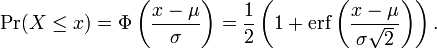
The normal distribution, also called the Gaussian distribution, is an important family of continuous probability distributions. It is applicable in many fields. Both in natural and social sciences. Each member of the family may be defined by two parameters, location and scale: the mean ("average", μ) and variance (standard deviation squared) σ2, respectively. The standard normal distribution is the normal distribution with a mean of zero and a variance of one. (Wikipedia)
The normal distributions are usually transformed into standard normal distributions. Then the calculations are performed.
The example
The following example is based on statistical applets provided by professor Charles Stanton at the California State University, San Bernardino. The original code is located here. I have modified and simplified the code. I have also arranged the window, in which we calculate the probabilities.
The next example consists of two files. The Normal.java and the Graph.java. We calculate the cumulative probability of the standard normal distribution. The input values are the mean, the variance and the score value x.
// Normal.java

import java.awt.BorderLayout;
import java.awt.Dimension;
import java.awt.GridBagConstraints;
import java.awt.GridBagLayout;
import java.awt.Insets;
import java.awt.event.ActionEvent;
import java.awt.event.ActionListener;

import javax.swing.BorderFactory;
import javax.swing.Box;
import javax.swing.JButton;
import javax.swing.JFrame;
import javax.swing.JLabel;
import javax.swing.JPanel;
import javax.swing.JTextField;


public class Normal extends JFrame {

    private Graph graph;
    private JPanel lpanel;
    private JTextField muField;
    private JTextField sigmaField;
    private JTextField xVal;

    private JLabel muLabel;
    private JLabel sigmaLabel;
    private JLabel xLabel;
    private JLabel pLabel;
    private JLabel result;


    private JButton calculate;


    public Normal() {

        setTitle("Normal Distribution");
        setDefaultCloseOperation(EXIT_ON_CLOSE);

        setLayout(new BorderLayout());

        graph = new Graph();

        graph.setPreferredSize(new Dimension(340, 340));
        graph.setBorder(BorderFactory.createEmptyBorder(50, 50, 50, 50));
        add(graph, BorderLayout.CENTER);


        lpanel = new JPanel();
        lpanel.setBorder(BorderFactory.createEmptyBorder(5, 5, 5, 5));
        lpanel.setLayout(new GridBagLayout());


        xLabel = new JLabel("x");
        xVal = new JTextField(5);
        xVal.setText("0");
        muLabel = new JLabel("Mean");
        muField = new JTextField(5);
        muField.setText("0");
        sigmaLabel = new JLabel("Std. Dev.");
        sigmaField = new JTextField(5);
        sigmaField.setText("1");

        pLabel = new JLabel("Cumulative probability: ");


        calculate = new JButton("Calculate");
        calculate.addActionListener(new ActionListener() {
            public void actionPerformed(ActionEvent event) {
                float x = Float.valueOf(xVal.getText());
                float mu = Float.valueOf(muField.getText());
                float sigma = Float.valueOf(sigmaField.getText());

                if (sigma <= 0) {
                    pLabel.setText("");
                    result.setText("Invalid Argument");
                    return;
                }

                graph.setSigma(sigma);
                graph.setMu(mu);
                graph.setValueX(x);
                graph.updateGraph();
                graph.repaint();
                if (pLabel.getText().isEmpty()) {
                    pLabel.setText("Cumulative probability: ");
                }
                result.setText(Double.toString(Phi(x, mu, sigma))
            }

        });

        JPanel sPanel = new JPanel();
        pLabel = new JLabel("Cumulative probability: ");
        sPanel.add(pLabel);
        result = new JLabel(Double.toString(Phi(0)));
        sPanel.add(result);
        add(sPanel, BorderLayout.SOUTH);

        GridBagConstraints c = new GridBagConstraints();
        c.gridx = 0;
        c.gridy = 0;
        c.insets = new Insets(3, 0, 0, 3);
        lpanel.add(muLabel, c);

        c.gridx = 1;
        c.gridy = 0;
        lpanel.add(muField, c);

        c.gridx = 0;
        c.gridy = 1;
        lpanel.add(sigmaLabel, c);

        c.gridx = 1;
        c.gridy = 1;
        lpanel.add(sigmaField, c);

        c.gridx = 0;
        c.gridy = 2;
        lpanel.add(xLabel, c);

        c.gridx = 1;
        c.gridy = 2;
        lpanel.add(xVal, c);

        c.insets = new Insets(25, 15, 0, 5);
        c.gridx = 0;
        c.gridy = 3;
        lpanel.add(calculate, c);

        add(lpanel, BorderLayout.WEST);
        add(Box.createRigidArea(new Dimension(20, 0)), BorderLayout.EAST);
        add(Box.createRigidArea(new Dimension(0, 20)), BorderLayout.NORTH);

        setSize(new Dimension(500, 250));
        setLocationRelativeTo(null);
        setVisible(true);
    }

    public static double erf(double z) {
        double t = 1.0 / (1.0 + 0.5 * Math.abs(z));

        double ans = 1 - t * Math.exp( -z*z - 1.26551223 +
                     t * ( 1.00002368 +
                     t * ( 0.37409196 +
                     t * ( 0.09678418 +
                     t * (-0.18628806 +
                     t * ( 0.27886807 +
                     t * (-1.13520398 +
                     t * ( 1.48851587 +
                     t * (-0.82215223 +
                     t * ( 0.17087277))))))))));

        if (z >= 0) return  ans;
        else        return -ans;
    }

    public static double Phi(double z) {
        return 0.5 * (1.0 + erf(z / (Math.sqrt(2.0))));
    }

    public static double Phi(double z, double mu, double sigma) {
        return Phi((z - mu) / sigma);
    }

    public static void main(String[] args) {
        new Normal();
    }

}
In the Normal.java file, we set up the layout of the window.
For this, we use the powerful
GridBagLayout.
float x = Float.valueOf(xVal.getText());
float mu = Float.valueOf(muField.getText());
float sigma = Float.valueOf(sigmaField.getText());
Inside the action listener of the calculate button, we get the three input values. The x, mean (mu) and the variance (sigma).
graph.setSigma(sigma);
graph.setMu(mu);
graph.setValueX(x);
graph.updateGraph();
graph.repaint();
Here we set three values for our graph and repaint it.
result.setText(Double.toString(Phi(x, mu, sigma))
The Phi(double z, double mu, double sigma) method returns the actual probability value.
public static double Phi(double z, double mu, double sigma) {
    return Phi((z - mu) / sigma);
}
Here we do the transformation into the standard normal variable.
public static double Phi(double z) {
    return 0.5 * (1.0 + erf(z / (Math.sqrt(2.0))));
}
The computation is based on the cumulative distribution function formula.
double ans = 1 - t * Math.exp( -z*z - 1.26551223 +
             t * ( 1.00002368 +
             t * ( 0.37409196 +
             t * ( 0.09678418 +
             t * (-0.18628806 +
             t * ( 0.27886807 +
             t * (-1.13520398 +
             t * ( 1.48851587 +
             t * (-0.82215223 +
             t * ( 0.17087277))))))))));
We use the Horner's method to calculate the error function.
// Graph.java

import java.awt.BasicStroke;
import java.awt.Color;
import java.awt.Graphics;
import java.awt.Graphics2D;
import java.awt.RenderingHints;
import java.awt.geom.AffineTransform;
import java.awt.geom.GeneralPath;
import java.awt.geom.Point2D;

import javax.swing.BorderFactory;
import javax.swing.JPanel;


public class Graph extends JPanel {


    float[] abscissa =
    { -4.0f, -3.9f, -3.8f, -3.7f, -3.6f, -3.5f, -3.4f, -3.3f, -3.2f, -3.1f,
      -3.0f, -2.9f, -2.8f, -2.7f, -2.6f, -2.5f, -2.4f, -2.3f, -2.2f, -2.1f,
      -2.0f, -1.9f, -1.8f, -1.7f, -1.6f, -1.5f, -1.4f, -1.3f, -1.2f, -1.1f,
      -1.0f, -0.9f, -0.8f, -0.7f, -0.6f, -0.5f, -0.4f, -0.3f, -0.2f, -0.1f,
      0.0f, 0.1f, 0.2f, 0.3f, 0.4f, 0.5f, 0.6f, 0.7f, 0.8f, 0.9f, 1.0f, 1.1f,
      1.2f, 1.3f, 1.4f, 1.5f, 1.6f, 1.7f, 1.8f, 1.9f, 2.0f, 2.1f, 2.2f, 2.3f,
      2.4f, 2.5f, 2.6f, 2.7f, 2.8f, 2.9f, 3.0f, 3.1f, 3.2f, 3.3f, 3.4f, 3.5f,
      3.6f, 3.7f, 3.8f, 3.9f, 4.0f };

    float[] ordinate =
    { 1.34E-004f, 1.99E-004f, 2.92E-004f, 4.25E-004f, 6.12E-004f, 8.73E-004f,
      1.23E-003f, 1.72E-003f, 2.38E-003f, 3.27E-003f, 4.43E-003f, 5.95E-003f,
      7.92E-003f, 1.04E-002f, 1.36E-002f, 1.75E-002f, 2.24E-002f, 2.83E-002f,
      3.55E-002f, 4.40E-002f, 5.40E-002f, 6.56E-002f, 7.90E-002f, 9.40E-002f,
      1.11E-001f, 1.30E-001f, 1.50E-001f, 1.71E-001f, 1.94E-001f, 2.18E-001f,
      2.42E-001f, 2.66E-001f, 2.90E-001f, 3.12E-001f, 3.33E-001f, 3.52E-001f,
      3.68E-001f, 3.81E-001f, 3.91E-001f, 3.97E-001f, 3.99E-001f, 3.97E-001f,
      3.91E-001f, 3.81E-001f, 3.68E-001f, 3.52E-001f, 3.33E-001f, 3.12E-001f,
      2.90E-001f, 2.66E-001f, 2.42E-001f, 2.18E-001f, 1.94E-001f, 1.71E-001f,
      1.50E-001f, 1.30E-001f, 1.11E-001f, 9.40E-002f, 7.90E-002f, 6.56E-002f,
      5.40E-002f, 4.40E-002f, 3.55E-002f, 2.83E-002f, 2.24E-002f, 1.75E-002f,
      1.36E-002f, 1.04E-002f, 7.92E-003f, 5.95E-003f, 4.43E-003f, 3.27E-003f,
      2.38E-003f, 1.72E-003f, 1.23E-003f, 8.73E-004f, 6.12E-004f, 4.25E-004f,
      2.92E-004f, 1.99E-004f, 1.34E-004f };

    Point2D.Float xdata[];


    int w, h;
    float a, b, c, d;
    float lowX, highX, lowY, highY;
    float x, y;
    float sigma, mu;

    BasicStroke curveStroke, thinStroke;

    public Graph() {

        setBorder(BorderFactory.createEmptyBorder(50, 50, 50, 50));

        xdata = new Point2D.Float[abscissa.length];

        sigma = 1;
        mu = 0;
        x = y = 0;

        for (int i = 0; i < xdata.length; i++) {
            xdata[i] =
                    new Point2D.Float(1 * abscissa[i] * sigma + mu, ordinate[i] /
                                      (float) Math.sqrt(sigma));
        }

        lowX = (float) xdata[0].getX();
        highX = (float) xdata[xdata.length - 1].getX();
        lowY = 0f;
        highY = 0.5f / (float) Math.sqrt(sigma);

    }

    public void paint(Graphics g) {

        Graphics2D g2 = (Graphics2D) g;

        RenderingHints rh =
            new RenderingHints(RenderingHints.KEY_ANTIALIASING,
                RenderingHints.VALUE_ANTIALIAS_ON);

        rh.put(RenderingHints.KEY_RENDERING,
               RenderingHints.VALUE_RENDER_QUALITY);

        g2.setRenderingHints(rh);

        curveStroke =
                new BasicStroke(3, BasicStroke.CAP_BUTT, BasicStroke.JOIN_ROUND);
        thinStroke = new BasicStroke(0.01f);

        w = getWidth();
        h = getHeight();

        a = w / (highX - lowX);
        b = -h / (highY - lowY);
        c = 15 - a * lowX;
        d = h - 30;

        AffineTransform tx;
        Point2D.Float p;
        GeneralPath path1, path2;


        tx = new AffineTransform(a, 0, 0, b, c, d);
        Point2D.Float[] transformed = new Point2D.Float[xdata.length];
        tx.transform(xdata, 0, transformed, 0, xdata.length);


        Point2D.Float x0 = new Point2D.Float(x, y);

        path1 = new GeneralPath();

        g2.setStroke(curveStroke);
        p = transformed[0];

        int i = 0;
        path1.moveTo((float)p.getX(), (float)p.getY());

        while (((i < xdata.length) && (xdata[i].getX() <= x0.getX()))) {
            path1.lineTo((float)p.getX(), (float)p.getY());
            p = transformed[i];
            i++;
        }

        path1.lineTo((float)p.getX(), (float)p.getY());

        Point2D.Float trans =
            new Point2D.Float((float)x0.getX(), (float)x0.getY());
        Point2D.Float temp = new Point2D.Float();
        tx.transform(trans, temp);

        path1.lineTo(temp.getX(), temp.getY());
        path1.closePath();

        path2 = new GeneralPath();
        i--;
        if (i < 0) i = 0;

        p = transformed[i];
        path2.moveTo((float)p.getX(), (float)p.getY());

        while ((i < xdata.length - 1)) {

            path2.lineTo((float)p.getX(), (float)p.getY());

            i++;
            p = transformed[i];
        }

        path2.lineTo(temp.getX(), temp.getY());
        path2.closePath();


        g2.setColor(Color.gray);
        g2.draw(path1);
        g2.setColor(Color.gray);
        g2.fill(path1);

        g2.setColor(Color.gray);
        g2.draw(path2);
        g2.setColor(Color.white);
        g2.fill(path2);
    }


    public void updateGraph() {
        for (int i = 0; i < xdata.length; i++) {
            xdata[i] =
                    new Point2D.Float(1 * abscissa[i] * sigma + mu, ordinate[i] /
                                      (float)Math.sqrt(sigma));
        }
        lowX = (float) xdata[0].getX();
        highX = (float) xdata[xdata.length - 1].getX();
        lowY = 0;
        highY = 0.5f / (float) Math.sqrt(sigma);
    }


    public void setValueX(float x) {
            this.x = x;
    }

    public void setSigma(float sigma) {
        this.sigma = sigma;
    }

    public void setMu(float mu) {
        this.mu = mu;
    }
}
The Graph.java class is responsible for drawing the graph. The abscissa is another name for the x-axis. The ordinate is another name for y-axis. The values in the arrays are used for drawing the normal probability distribution.
a = w / (highX - lowX);
b = -h / (highY - lowY);
c = 15 - a * lowX;
d = h - 30;

...

tx = new AffineTransform(a, 0, 0, b, c, d);
An affine transform consists of three parts. The scaling factor, the shearing factor and the translation factor. The a, b values stand for the scaling factor and the c, d values stand for the translation factor.
tx = new AffineTransform(a, 0, 0, b, c, d);
Point2D.Float[] transformed = new Point2D.Float[xdata.length];
tx.transform(xdata, 0, transformed, 0, xdata.length);
Every time the window is resized an affine transform is done. We reflect the current height and width of the panel, on which we draw the graph.
path1 = new GeneralPath();

g2.setStroke(curveStroke);
p = transformed[0];

int i = 0;
path1.moveTo((float)p.getX(), (float)p.getY());

while (((i < xdata.length) && (xdata[i].getX() <= x0.getX()))) {
    path1.lineTo((float)p.getX(), (float)p.getY());
    p = transformed[i];
    i++;
}

path1.lineTo((float)p.getX(), (float)p.getY());

Point2D.Float trans =
    new Point2D.Float((float)x0.getX(), (float)x0.getY());
Point2D.Float temp = new Point2D.Float();
tx.transform(trans, temp);

path1.lineTo(temp.getX(), temp.getY());
path1.closePath();
The graph is created with two general paths. The first is the gray part of the graph, which represents the cumulative probability. The second one is the rest.
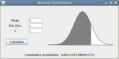
In this chapter, we have created a program which calculates the calculate cumulative standard normal probability.